Structured programming is a disciplined approach to programming that results in programs that are easy to read and understand and are less likely to contain errors. Structured programming was developed in the 1960s and has become so well accepted since that time that almost nobody attempts to write programs any other way. We hope you agree that the programs written so far are relatively easy to read and understand.
Structured programming comes from a systematic approach to stating complex problem solutions in terms of sequences of subtasks, selections among several alternative subtasks, and repetitions of subtasks. To illustrate that this is a natural approach even if the problem is not being solved on a computer, we consider first an example from everyday life.
Case Study: Changing a Flat Tire
You are driving a car with two friends and suddenly get a flat tire. Fortunately, there is a spare tire and jack in the trunk.
After pulling over to the side of the road, you might decide to subdivide theproblem of changing a tire into the subproblems below.
Algorithm
2. Loosen the lug nuts from the flat tire and remove it.
3. Get the spare tire, place it on the wheel, and tighten the lug nuts.
4. Lower the car.
5. Secure the jack and flat tire in the trunk.
Because these steps are relatively independent, you might decide to assign subproblem 1 to friend A, subproblem 2 to friend B, subproblem 3 to yourself, and so on. If friend A has used a jack before, the whole process should proceed smoothly; however, if friend A does not know how to use a jack, you need to refine step 1 further.
Step 1 Refinement
1.1. Get the jack from the trunk.
1.2. Place the jack under the car near the flat tire.
1.3. Insert the jack handle in the jack.
1.4. Place a block of wood under the car to keep it from rolling.
1.5. Jack up the car until there is enough room for the spare tire.
Step 1.4 requires a bit of decision making on your friend's part. Because the actual placement of the block of wood depends on whether the car is facing uphill or downhill, friend A needs to refine step 1.4.
Step 1.4 Refinement
1.4.1. If the car is facing uphill, then place the block of wood in back of a tire that is not flat; if the car is facing downhill, then place the block of wood in front of a tire that is not flat. This is actually a selection action: One of two alternative actions is selected, depending on a certain condition.
Finally, step 1.5 involves a repetitive action: moving the jack handle until there is sufficient room to put on the spare tire. Often, people stop when the car is high enough to remove the flat tire, forgetting that an inflated tire requires more room. It may take a few attempts to complete step 1.5.
Step 1.5 Refinement
1.5.1. Move the jack handle repeatedly until the car is high enough off the ground that the spare tire can be put on the wheel.
The algorithm for changing a flat tire has three categories of action: sequential execution, conditional execution, and repetition. Sequential execution simply means to carry out steps 1.1 through 1.5 in the sequence listed. Step 1.4.1 illustrates selection in that placement of the block of wood depends on the angle of inclination of the car. Step 1.5.1 illustrates repetition.
Structured programming is a way of carrying into computer programs the natural method of systematic problem solving just described. Structured programming utilizes control structures to control the flow of statement execution in a program. There are three kinds of control structures: sequence, selection, and repetition or iteration. So far, each program we have looked at has consisted of a sequence of individual statements, and the flow of control has been passed from one statement to the next, beginning with the first statement in the program body and ending with the last statement in the program body.
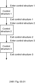
In the next few chapters, we will introduce some Ada control structures. The control structures of a programming language enable us to group a sequence of related statements into a single structure with one entry point and one exit point. We can then write a program as a sequence of control structures rather than as a sequence of individual statements (see Figure 3.1).
Figure 3.1

So far we have extended the solution to one problem (find a circle radius and circumference) into a second related problem (find the unit price of a pizza). We are not really finished yet because our goal was to be able to do a cost comparison of several pizzas with different prices and sizes in order to determine the best value.
One way to accomplish our larger goal is to run this program several different times, once for each pizza, and record the results. Then we can scan the list of results to determine which pizza has the lowest unit price.
A better solution would be to write a program that repeated the computation steps and also compared unit prices, displaying as its final result the size and price of the pizza with the lowest unit price. Let's write an algorithm that will give us this improved solution.
Initial Algorithm for Improved Solution to Pizza Problem
1. For each size of pizza, read in the pizza size and price and compute unit cost. Compare the unit cost just computed with the previous unit costs and save the size and price of the pizza whose unit cost is the smallest so far.
2. Display the size and price of the pizza with the smallest unit cost.
The purpose of step 1 of the algorithm is to perform the cost computation for each individual pizza and somehow save the size and price of the pizza whose unit cost was the smallest. After all costs are computed, step 2 displays the size and price of the pizza that is the best buy.
We don't know how to do step 1 yet in Ada because it involves the use of repetition and selection control structures. However, we can write a refinement of this step that will give you some idea of where we are heading in the next few chapters.
Step 1 Refinement
1.1. Repeat the following steps for each size of pizza:
1.2. Read in the next pizza size and price.
1.3. Compute the unit price.
1.4. If the new unit price is the smallest one so far, then save this pizza's size, price, and unit price.
Step 1.1 specifies the repetition of a group of steps: step 1.2 (read), step 1.3 (compute), and step 1.4 (compare). We will repeat these steps as many times as necessary until all unit prices are computed. Each time we compute a new unit price, step 1.4 compares it to the others, and the current pizza's size and price are saved if its unit price is smaller than any others computed so far. If the unit price is not the smallest so far, the current pizza's size and price are not saved. Step 1.4 is a selection step because it selects between the two possible outcomes--(a) save the pizza's data and (b) do not save the pizza's data.
We will discuss control structures for selection and repetition further in Chapters 4, 5, and 6.
Copyright © 1996 by Addison-Wesley Publishing Company, Inc.